P&L and B/S forecasting intro

Companies of all sizes do financial accounting, which is the standard practice. Most companies worldwide align their accounting systems with principles like IFRS (International Financial Reporting Standards) or GAAP (Generally Accepted Accounting Principles). While simpler methods exist, taxes are typically calculated based on these standards, so most companies follow the same rules.

Backend systems, such as SAP, record all financial transactions in a vast database. Using this data, financial analysts summarise a company’s performance and health into two key reports that their management frequently uses: the P&L (Profit and Loss) statement and the B/S (Balance Sheet).

• P&L Statement, also known as an income statement or statement of operations. This report summarises a company's revenues, expenses, and profits or losses over a specific period, such as a fiscal year, a quarter, or on a rolling basis, monthly. It highlights a company's ability to generate sales, manage costs, and create profit, making it a critical document for investors.
• Balance Sheet. This is a financial statement that provides a "snapshot" of a company’s financial health at a specific moment in time. It lists the company's assets, liabilities, and shareholders' equity. It is essential for investors, lenders, and management to assess a company’s financial position, solvency, and future growth potential.

Both reports are vital, offering two different perspectives on a business's health.

There are multiple software systems helping companies to generate these reports (EPM, Enterprise Performance Management software). Some of these systems also provide basic or advanced systems for Financial Statement forecasting.

The Challenge of Forecasting

Depending on the ability of the company, these reports are produced yearly (mandatory by regulators), quarterly or monthly. Theoretically, it could be possible to check the status weekly or even daily, but in practice, this doesn't work. Having frequent updates, management can control trends better, and as the business becomes more complex, it appears to be more important.

The standard reporting is essential. However, it always shows a precise picture of the past. These reports allow analysts to trace figures and understand the reasons for success or, more often, failure (mainly second, of course, to find the guilty employee). It is also possible to make a mind experiment: let's assume it will go as it went before, thus we will come to this and that result. This type of experiment is called nowadays "data-driven decision". However, this approach has limitations. If you change your perspective to the past 3 months or 33 months, the linear trend can change dramatically. It is also a question: how far into the future can this trend be expanded? One month? Quarter? 7 years?

Again, this works for a simple business. The complex one depends on too many drivers that no-one is able to keep in their head. Thus, finance management requires AI-driven prediction.

Traditional finance professionals are often sceptical of AI predictions because their work is based on real, verifiable facts. Every financial transaction generates many financial implications spread over the company in financial streams and then summarised at the end in the report. They believe that without knowing every future detail - such as when a contract will be signed, a product delivered, or an employee hired or fired, how the contract will be modified, and the inflation rate will be changed - it’s impossible to guarantee an accurate forecast.

It will be like a crystal ball, nothing more.

This is why traditional FP&A (Financial Planning & Analysis) departments often produce forecasts based on broad assumptions, which can deviate from reality by a significant margin.

Experimentational finance professionals understand the complexity of forecasts and attempt to use various techniques. Unfortunately, over the years, the MS Excel approach skewed their mind to spreadsheet thinking. Therefore, multiple limitations of Excel are assumed as "natural limits" and, in many cases, prevent freedom in thinking.

Data scientists have a different perspective. They don't aim to track every single transaction but rather to aggregate them so that they follow patterns a machine can identify. While these rules aren't "exact" and there is always some uncertainty, they can guarantee that the level of error won't exceed a predetermined, acceptable limit — for example, the same margin of error as a manual forecast. Data engineers help to connect various data sources and, therefore, to build a near-real-world model for better predictions.

What will be the benefit then? Actually, two.

1. Efficiency and Resource Allocation: Analysts can be freed from the tedious task of creating forecasts. This might seem minor for a small business, but for a large multinational corporation, it could allow for the reallocation of hundreds of high-skilled employees to more strategic work. 500*yearly salary=?
2. Speed and Agility: A machine can complete a full forecasting cycle in a couple of hoursinstead of a month. This means management can get an end-of-year P&L on January 1st instead of February 1st and year-forward forecast the same day — do you feel the difference? This speed also allows for nearly real-time scenario planning. A manager can adjust various drivers like labour costs, FTE count, inflation, or competition and receive an updated forecast within hours. This allows assessing the sustainability of the company, the business's stability, and effectively managing risks.

We will try to highlight HOW to make this forecast available as a service.

Granularity, time, changes in business: all about raw data

Every Data Science project starts with data. Sounds obvious — but in practice, this is where most projects fail. Before jumping into Python notebooks or neural networks, there are fundamental questions that must be addressed. Here are a few we always start with:

1. Do we have at least the basic data? For P&L and B/S forecasting: can we trace the data back in time? Are reports complete for previous periods? What is the frequency and schedule of updates?
2. What is the granularity of the data? How deep can we investigate: by markets, business units, reporting structures? What granularity is needed for training vs. forecasting? (They are not always the same.)
3. What is the backward horizon? How far back does the history go, and how reliable is it? Can we trust older data? What is the required forecasting horizon?
4. Do we have a forecasting basis beyond time? Are there variables such as sales, inflation, or contracts? What is their horizon, granularity, and update frequency?
5. What about external data? Do we plan to use it? Do we have access? What is its refresh rate and granularity?

Let’s say management decides to go ahead with P&L forecasting. If we struggle to answer questions like:

• Who owns the relevant data sets?
• How do we get access?
• Who can explain how the data was derived?

…then maybe it’s time to pause or STOP the project. Yes, a Data Scientist can come up with personal answers, but unless those answers are confirmed and accepted by SMEs, managers, and stakeholders — they are worthless. These aspects must be locked into the Project Charter and made visible to everyone.

It is very important to have access to SMEs for all business units, territories and reporting elements throughout the project. They are a valuable source of information about the company data.

The time dimension

Usually, the history length is a common obstacle. Seven years of yearly P&L reports? Useless - you can only draw a linear trend through seven points in Excel. Even monthly data for just three years gives 36 observations - meaningless for training a neural network.

The geo/business dimension

From my experience, the forecasting of P&L at corporate level is “easy” - but also pointless (and, to be honest, is performed by every investor regurarly). Aggregation smooths everything out, making it close to constant. The gain of one business compensates the other business loss. Change on a weak market is just a small abberation on the surface of huge markets like China or USA.

Real insight requires detail: by channel in every country and for every product ID. Unfortunately, at this level, volatility often looks like pure white noise. Choosing the right level of granularity requires serious preliminary research and, again, deep SME involvement.

The report line dimension

A published P&L or B/S usually has 15–20 lines. However, each can be broken down further... and provide more insights and better understanding of company business, and even deeper. The analyst can end up finally at the FSI (Financial Statement Item) - the low level attribute of the transaction in the financial system.

Forecasting at this lowest level sounds attractive, but business rules change constantly. Every FY brings new FSIs and terminates accounting at previous FSI groups. And, what is the worst: employees who knew everything about 3-year-old FSIs are fired already. Thus, again the Data Scientist should first do a study and choose the right level of aggregation.

The takeaway: Even when a project is formally initiated, resist the urge to dive straight into coding. A huge amount of work must happen first: defining scope, aligning with SMEs, validating data ownership, and deciding on the right level of aggregation. Skipping this step is the fastest way to doom a project before it even starts.

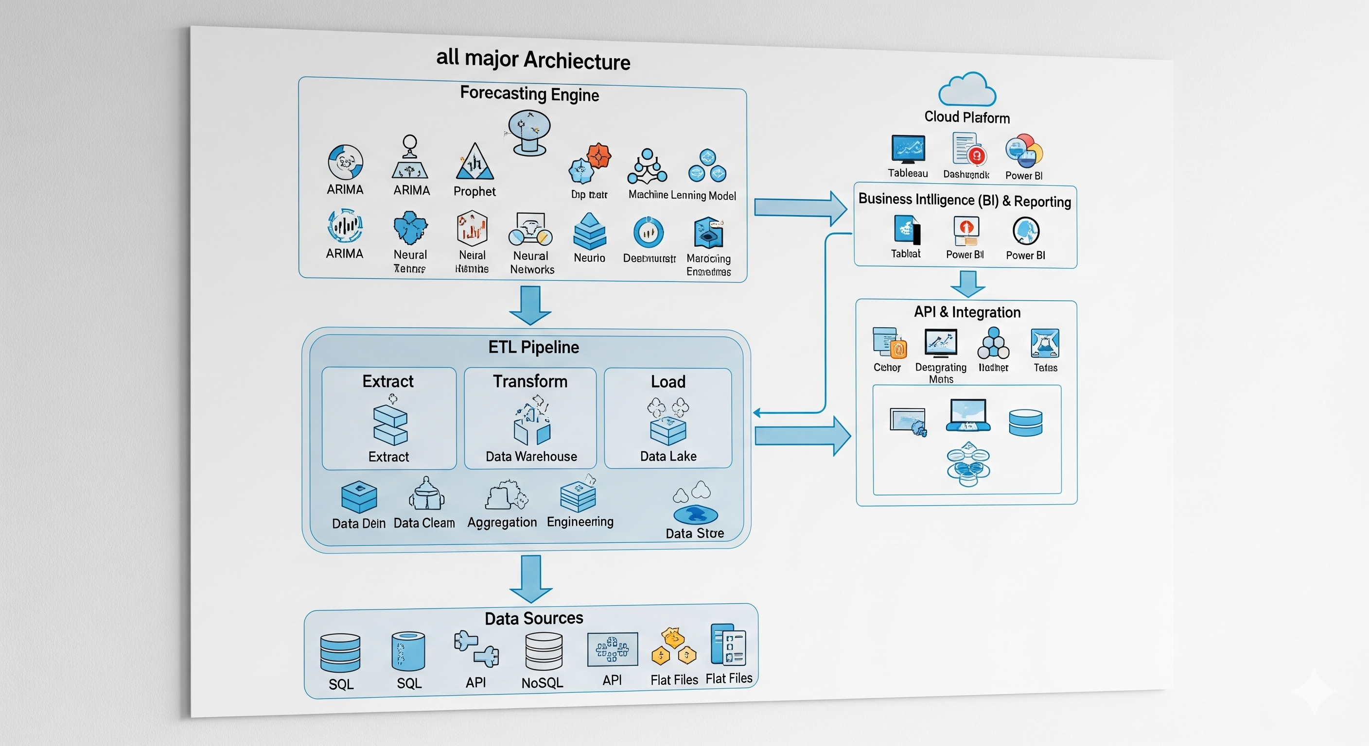
The Architecture of a Forecasting Solution

So, we’ve decided about the right data for our ambitious P&L or B/S forecasting project and are eager to start coding the first ETL pipeline. But hold on. Not so fast.

Before we rush into coding, let’s step back and think about the overall architecture. What are the three non-negotiable requirements?

1. No human in the data input loop

All data must be available in the correct databases before the system kicks off re-training. This requirement applies not only to data formats but also to the surrounding business processes. The ETL pipeline must work seamlessly on demand, ideally triggered automatically by the system itself, not a human pressing buttons.

2. Automated re-training with minimal human intervention

The solution should be capable of retraining itself. Yes, a data scientist should step in when something breaks beyond repair, but in most cases the training cycle must self-correct errors in both data and code.

3. Zero dependency on technical staff for delivery

Forecasts must reach end users directly - no more bottlenecks of Excel exports or PowerPoint updates. Results should flow instantly into self-service BI tools so decision-makers can act on them immediately.

Well, even before a single line of code, we face a host of IT design choices:

• Where will the code run?
• Where does the data live, and does the executor system have continuous, secure access? What about security rules: how to avoid expiration of rights, for example?
• Is data access fast enough, or do we replicate it closer to the compute?
• What facility will schedule re-training?
• Which BI tools do finance teams actually know and have access to?
• Can the core executor deliver results directly into those BI tools without manual handling? Again: how do we deal with access rights that may expire?
• and many more

Only after answering these questions does the final consideration emerge: what language to use? Python is good, but depending on the architecture, we perhaps choose pure SQL, a no-code solution, or even something else entirely.

The bottom line: Architecture is strategy. Code is just execution. 

P&L Forecasting Approaches: ARIMA, ML, NNet and more

Well, we shaped the solution: the Project Charter approved, the source data topics resolved, the architecture is ready, and finally, we’ve chosen a language to code!

We could already start programming the ETL, but let’s take a pause and think about the general approach to the forecasting kernel of our system. Cool down and decide: what statistical method should we apply?

I would say, there are four general modelling approaches.

1. Rule-based forecasting

A Data Scientist can fully rely on the experience of finance colleagues and simply code the rules they used before. These rules may look strange, but they often work — some have worked for years, and you can just leave them as they are.

This approach doesn’t require any ML knowledge. In fact, the company doesn’t even need a Data Scientist; a smart manager with Python skills (and ChatGPT at hand) could create such a solution nowadays.

Two issues:

• It is often very difficult (or impossible) to extract these rules from financial analysts.
• Once coded, the rules cannot evolve with data.

The only benefits are execution speed and the possibility of removing the expert from the loop.

However… see also approach 5*.

2. Auto-regressive models (ARIMA)

One can apply ARIMA to derive the next period from the past behaviour of a time series — cyclical waves, trends, and seasonalities. With long historical series, this can yield very precise short-term predictions.

The limitation: the forecasting horizon. It is usually similar to traditional manual forecasts and deteriorates quickly into the future.

3. Machine Learning techniques

A Data Scientist can employ ML methods such as linear regression, polynomial regression, GAM, decision trees, XGBoost, and many others. Each has limitations and requires careful data preparation and feature engineering. Development and testing can be time-consuming.

The advantage over ARIMA and NNet: you can easily derive feature importance and provide more transparent scenario forecasts that business users can understand.

4. Neural Networks

The beauty of this approach is that you can feed everything into the NNet — it will handle factor selection, some feature engineering, and accuracy testing in one run. In theory, you don’t even need SMEs.

The drawback: SMEs will never trust the forecast, since it is a black box. Scenario forecasting is possible, but results can be unstable for rare or out-of-scope values.

5*. Hybrid and hierarchical approaches

And, of course, we arrive at the mixture of all the above. This is especially relevant for P&L and B/S forecasting.

As explained earlier, dimensions such as geo, business, and report items can be decomposed into buckets. In practice, it’s normal to have 5,000–25,000 buckets. You can treat them as independent processes and model each separately.

Then, you sequentially introduce different approaches (1 through 4). For a given bucket, you may test multiple methods, then hold discussions with SMEs to assess feasibility in a multidimensional decision space (accuracy, maintainability, adoptability).

Two possible strategies:

• Use a universal “Swiss knife” model across all buckets.
• Assign different methods to different buckets.

If IT can maintain diverse code, and in case of general acceptance by stakeholders, it’s worth either:

• building an automatic selector of the best statistical method per bucket, or
• using an ensemble of methods and returning a consensus forecast (though good luck explaining that to finance!).

A final note on method selection As mentioned, splitting into buckets produces thousands of “independent” time series. But in reality, business units often reallocate budgets across markets or products, and accounting has some (limited) flexibility in FS item categorisation.

At a high level of aggregation, data is usually stable and can be predicted with simple models like a constant or linear trend. If we have, let's say, 100 simple models at level H1 for buckets aggregated at <FSI_lev1, BIZ_lev1, GEO_lev1>, we can predict the future and use this prediction as an additional engineered factor for the next, deeper, level of aggregation H2, buckets <FSI_lev1, BIZ_lev2, GEO_lev1>. We can utilise this kind of hierarchical descent to make interconnected forecasts for all buckets at any level.

At each H*, for each bucket, we are free to choose any of the methods described above (1–5*).

Features for ML and NN (internal, external, feature engineering)

Perhaps, we decided to follow approach #5*: a mix of the other approaches. Let’s dive into the modelling process now. This post is dedicated to features; the next one will cover methods.

For every bucket, we create a data table with one row per observation and a column for every feature. One of the columns will be used as the target variable, the one we want to predict. All columns in our data table are filled with values - both for the past and the future. We train the model on the dataset up to the current period (month) and run the predict() function for rows from the current month into the future.

Therefore, the number of rows in our data table equals (length of history) + (forecast horizon). The number of columns is at least one. (See also the next post - length of history can be expanded).

We can use three types of features to fill in other columns: internal data, external data, and engineered data.

Before adding features: analyse the target variable

I think it would be a good idea to look over the target variable first. There are many situations where you don’t need a complex model at all:

• the target variable is constant (or almost constant);
• the target variable has no values in the last half year (though it had them before);
• it is not constant, but shows just one-off allocations (e.g., +1M EUR in January and -1M EUR in February);
• etc.

This rule-based control can save a lot of electricity. Up to 30% of buckets can be predicted as simple constant values. This stage is also the right time for handling outliers. As in the third example above, such situations are very frequent in accounting, even if FSI is in use. A Data Scientist can create rules to detect these allocations and smooth them by summarising peaks across consecutive months.

Internal data

Now, let’s talk to stakeholders and SMEs. Perhaps:

• Sales already has a sales plan
• Marketing builds a demand forecast for two years
• S&OP has the Order Intake plan
• HR has headcount and salary increase plans (even by grade)

If this is the case, it significantly facilitates your job. First, it means other smart teams have already shaped the future using a variety of techniques — and you can base your model on that. Second, you shift 50% of the responsibility onto other departments. ;-) Often, you can even explain model failures by proving that “it was the incorrect sales forecast.”

Internal data is the most important knowledge about your business.

Example columns we added:

sales
OIT
demand
salary_50, salary_100 (by grade)

all with actual historical values and future figures from other departments, if available at the same granularity as our model. Otherwise, our data table may still only have one column (target variable).

External data

Now, let’s think about the business environment. A company is not isolated from legislation or the general economic situation. There are taxes and tariffs, commodity price fluctuations, and freight costs.

Many organisations provide both historical and forecasted figures for useful indicators. One can check World Bank or IMF (free APIs, [see post #2]), or paid services like Reuters, Bloomberg, NASDAQ (to be sure that the data was verified).

Example columns:

inflation
unit_labor_cost
labor_productivity
commodity_steel_price
etc.

Feature engineering

Now, we apply transformations to our data. Some are obvious, others look funny but still work. Here are just a few ideas:

sales2 = sales^2
sales_sqrt = sqrt(sales)
sales_log = log(sales)
sales_cum3M = last 3 months running sum
sales_diff = difference
sales2_diff = difference of squared sales
sales_1M, sales_4M = sales shifted by 1 and 4 months
sales_3M_trade = sales_cum3M / sales_cum3M_1M
OIT_1M, OIT_7M
OIT_MoM = month-over-month change
inflation_MoM
labor_productivity_MoM

Such variables arise from the analysis of dependencies between the target and transformations of existing variables. Differentials and cumulative values are particularly useful for the Balance Sheet because it contains cumulative figures. Thus, we either differentiate before forecasting or integrate features.

⚠️ Note: if we struggle to obtain internal or external variables, then we also have no engineered ones, and our data table remains with only the target variable.

Time-based features

So far, none of our features has been explicitly linked to time. Assuming we use monthly reports (rows = months/periods), we can add:

monthID = 1...12
monthID2 = monthID^2
monthID_log = log(monthID)
quarter

Yes, it is the linear component, but our business usually near-linearly grows, thus this linearity would be helpful for regression models.

Self-target features

We can also derive three new features from the target variable itself:

1. 12-month pattern. Even without future values, we can estimate how the FSI for this bucket changed within each year and build an averaged 12-month pattern. A minimally tuned ARIMA can be used. This pattern can be replicated across the dataset and help the modelling engine.
2. Event markers.It is worth including the additional factor for unexplained situations. Basically, there are some explanations: acquisition of other businesses, huge payouts because of lost court cases, and many more. It looks like an enormous peak in P&L FSI, or like an enormous jump in values in B/S FSI. Such situations can be detected automatically; they are rare, and therefore we can introduce the special feature that equals 0 all the time, and 1 in the month of the event - for P&L; and it equals 0 before the jump and then 1 after the event - for B/S. This variable helps a lot to the linear regression procedure. It will be automatically added to the equation, and the rest of the values will be adjusted.
3. Hierarchical descent. Already mentioned earlier, but we can’t fill values at the feature engineering stage. We’ll cover this in the next section.

ML for Successful P&L and B/S Forecasts

In this section, we want to cover some additional aspects of modelling that weren’t included in the previous parts.

Weighting

The business of any company does not repeat itself every year. New products appear, the competitive environment changes, marketing methods evolve, and legislation introduces new boundaries.

So, when an SME gives you a sceptical look after you proudly say: “We use 20 years of historical reports, that’s 240 reliable data points” - don’t be surprised. In today’s world, everything changes so fast that even a 5-year-old P&L looks like a dinosaur. If you add: “My Machine knows about the business 7 years ago and still learns from it” - that’s a direct way to be kicked out of the room by the FP&A Director.

From a Data Scientist’s perspective, however, losing this information is painful. Fortunately, smart people invented weighting: a vector of values assigned to every period. In simple terms, it defines the probability that past information is still relevant to today’s reality.

Human forecasts

So far, we’ve used only actual historical data. But there’s another source. It’s disputable, but hear me out.

A few years ago, dozens of financial analysts in your company worked on P&L and B/S forecasts. They spent enormous effort analysing the future (which, for us, is already the past) and producing their best estimates. That is also data. It is the unrealised version of reality.

If FP&A produced forecasts quarterly, then you already have significantly more data points. Why not include them in your dataset? You can add them as extra rows with low weights. These forecasts can also help establish stronger linkages between variables and teach the Machine.

Hierarchical descent

We already explained the reasoning behind hierarchical descent. But how do we actually build it?

While there are automated methods, I prefer a simpler and more flexible approach.

1. Start at the top level. Create a data table for consolidated P&L or B/S at a high aggregation level. The choice is yours, but buckets should remain stable over the years. For example, all FS items related to Liabilities in Europe for an entire business division. Train an ML model on the historical data, then run x = predict() for the full history and forecast horizon.
2. Go one level deeper. Split Europe into individual countries. Add this new x as a feature column to the data table - values are the same across countries (but vary by FSI and business, of course).
3. Continue descending. Use results from the previous level when modelling more detailed buckets, such as FS sub-items.

You define the number of steps and the final level of granularity.

Method selection

We decided to try different methods, without knowing upfront which one is best for each bucket. Let’s assume we test four:

• Stepwise Linear Regression or Lasso Regression
• Generalised Additive Model (GAM)
• XGBoost
• Neural Networks

How do we choose? By running each model and selecting the optimum within the metric space <accuracy, outliers, boundaries>.

• For accuracy, you can apply RMSE or similar metrics.
• For outliers, check the frequency and magnitude in forecasts.
• For boundaries, ensure stability. Some models (like GAM or NNets) may produce extreme values if features fall slightly outside the training scope. This is critical since we are modelling the future.

One model vs. ensemble

Finally, should we pick one model per bucket, or use an ensemble?

An ensemble — averaging predictions across models - can work like a “consilium of analysts.” But the drawback is that the developer will struggle to explain to stakeholders how the final result was obtained and what the main drivers were. Transparency often suffers.

Delivery of the P&L forecast (downstream)

The ML model returns vectors of data. However, for proper consumption, this data must be reshaped and delivered to end users. The proven way is via a BI tool.

The software development team should either prepare an extension to the existing P&L (B/S) reporting dashboard or design a new one based on existing templates. The main idea here: results must be delivered in tables familiar to finance colleagues. The Finance Department is one of the most conservative units in any company. They are used to working with huge tables (and their superpower is spotting errors or deviations in 0.5 seconds). But any change in the format makes them stuck.

It is quite difficult to explain what you meant by preparing a super-attractive chart for Finance colleagues. One or two lines on a chart are OK, but not more. A scatterplot diagram, widely useful for linkage detection, is simply out of scope for Finance. Therefore, tables in all shapes and forms, with dozens of filters here and there, remain the key.

By the way, Power BI has done a great job of designing everything in the way finance people love.

Finance professionals also love to extend their tables with additional metrics and KPIs. Every analyst has their personal “magic toolbox,” which is why they cannot survive without MS Excel. Thus, don’t limit their imagination - make export available.

Scenarios

As soon as we complete the main part of the project, we will have:

1. Delivered exactly what the Finance Department wants.
2. Organised the data flow process: from ETL, to auto-modelling, to presentation of results.
3. Orchestrated the architecture and made the solution flexible enough.
4. Enriched data with internal and external features.
5. Made ML models work.
6. Added power with additional data and business knowledge.
7. Prepared reporting in the form of self-service analytics.

So now we are ready to extend the system with business scenarios and optimisation capabilities.

Scenarios allow us to run the full predictive model under the assumption that any subset of drivers changes. The major limitation here is, of course, the boundaries of the training data. In theory, any value between max and min can be used because most statistical methods used for modelling are continuous. But internally, models like GAM can build cubic (x³) dependency functions and, as a result, even a small step into unobserved territory can potentially return too-large values.

All drivers can be distinguished as manageable and unmanageable. The latter includes factors such as inflation or labour cost. It is a useful exercise to run the model for various values of such drivers: the system will show the company’s resilience to external shocks.

Manageable drivers, in contrast, can be changed by the company’s management. For example, we can decide to increase sales in one market or reduce FTE in another. How will these actions influence the overall Balance Sheet or P&L? With this tool, we can proactively manage investor expectations.

If we are able to set the correct KPI, we can even run this scenario multiple times (automatically, millions of times) to find the right combination of manageable driver values, and identify the optimal path to company prosperity.

Is the business fully managed by AI now? Yes and no. This is just a recommendation, backed by figures. Whether this recommendation is acceptable to ExCo depends on how much they trust the system that they themselves initiated the development of.

And with this, we return to the start. We would recommend to Finance and company management think twice at the start of the project. Are you ready to share the drive wheel with AI?